A History of Server Application Deployment: Traditional Deployment

We all know there are servers somewhere running various programs. Some of us are familiar with virtual machines, and some may have even heard about containers – not the shipping kind, but those focused on OS-level virtualization. However, few understand how these technologies evolved, why they developed the way they did, or whom to credit for it. So, I decided to dive into it myself and share my findings with you. That’s why I’ve started this “Deployology” column.

Deployology – a term I just coined – is the science of deploying server applications. The process of deploying server applications, however, has been around for some time. It encompasses the setup, configuration, and activation of software components in a computing environment. Simply put, it’s all about putting code in the right place to make it run – in our case, on a server.

In this first part, I’ll cover traditional deployment, whose history closely parallels the broader development of computing. I’ll focus on the most significant milestones from my perspective. The next article will explore virtual machines on servers, and the third will dig deeper into containers, a topic I find particularly intriguing. Note that this division is more of a guideline, given the intertwined evolution and cross-influence of these technologies.

Traditional Teployment

1940: The Beginning

In the 1940s, at the dawn of computing, programs weren’t written and tested in editors, as they are now, but rather on paper and in the minds of programmers — or, as they were called back then, "computer mathematicians." The program was then manually translated into machine code. Operators would then enter the code and data into the computer using a myriad of switches and switching cables on plug-in panels; there were no other input devices. The process of entering a tiny program into such systems could take hours to days, during which time the computing facilities were idle. Maintenance and operation of electromechanical computing machines of that time required patience and attention from the personnel. At times, good physical fitness was required, as the photo below illustrates. It can be seen that in order to enter a new program into the machine they had to do a lot of squats and bends.

Subsequently, data began to be entered into calculators using punched cards. Creating and checking them were also very labor-intensive processes requiring special equipment. However, this significantly relieved operators and increased the speed of data processing.

Computing machines of that time were often unique products solving a narrow range of tasks and could differ radically from each other in their design and programming methods, requiring specialized knowledge. Transferring a program from one machine to another was hardly less complicated than writing a program from scratch. But despite all the complexities of the work, the efficiency of computing machines seemed incredible for that time.

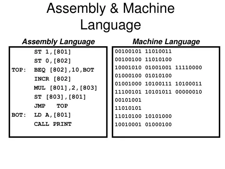
1947: Assembly Language

Writing programs in machine code is an extremely inconvenient process that requires knowledge of the architecture and specifics of a particular computing machine. To simplify programming and increase the level of abstraction from the "hardware", low-level programming languages were developed. Using special commands that are more understandable and convenient for humans, these languages became the first step in the direction of increasing the efficiency of programming.

At the first stages of development low-level languages differed significantly for different computing machines, and they were called autocode, basic order set, initial orders. Then some unification took place and the name "assembly language" or assembly language appeared. To convert assembly language code into machine code, a translator program called assembler was used.

The first assembly language was developed by Kathleen Booth in 1947 for the ARC2 computer.

Programs written in assembly language are unambiguously translated into instructions of a particular processor and can be transferred with some modifications to run on machines with a different instruction system. This has increased the portability of programs and the versatility of computing machines, simplified and accelerated the development and deployment of programs.

1949: Downloading Saved Programs

Typing the program anew each time it was reconfigured for another task was a rather laborious and time-consuming process. At the same time, data input from punch cards was significantly faster and more efficient, although it was associated with quite a large number of reading errors. The idea arose to load programs from removable media as data, leaving only the initial sequence of commands in the iron logic, similar to a modern BIOS. The initial sequence of commands should ensure that the next portion of the program would be read from a replaceable storage medium, such as punched cards or punched tapes. This approach was applied for the first time in 1949 on the EDSAC computer, which at that time was still called a "calculator".

The error rate for data input from the first punch cards could reach several percent of the total data, which was unacceptably high, especially for the control program code. To solve this problem, important data could be repeated, and the system signaled an input error if their inputs diverged. Data integrity checks, error control and data recovery tools were also introduced.

Reading the program from the medium allowed to quickly reconfigure the computer for different tasks, significantly reducing the downtime and allowing easy transfer of programs between machines. An important advantage of punched cards was the possibility of their copying. In modern computing, the storage media have changed, but the overall approach has remained the same.

1957: High-level Programming Languages

Low-level programming languages allowed to effectively use hardware capabilities of computing machines, but at the same time they had significant disadvantages. The code in low-level languages was inconvenient to understand, difficult to debug and maintain, which significantly slowed down the process of developing new software and making changes to existing software. Low-level languages strongly depended on hardware and differed for different machines, which required modifications when transferring to machines with different architecture and understanding the specifics of "hardware". To increase the speed of software development and increase its complexity, a language with a higher level of abstraction was required, which would lower the threshold of entry and allow less delving into the intricacies of hardware.

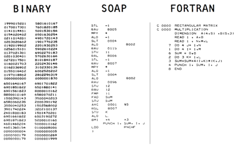
The first high-level language was Plankalkül, which translated from German meant planned calculations. The language was developed in 1945 in the then Nazi Germany by engineer Konrad Zuse for the Z4 computer. However, Plankalkül did not become a massively used language and was not developed because of Germany's defeat in the war and the difficulties in restoring the Z4 in post-war Europe.

And the really mass high-level language was Fortran, developed in 1957 by a group of programmers led by John Backus at IBM. The name Fortran is an abbreviation of FORmula TRANslator - formula translator, which reflects the goals that were pursued during its development - simplification of mathematical calculations to solve scientific and engineering problems.  Fortran made it easier to port programs to different platforms through rigid standardization and made programming much easier, allowing the creation of complex programs while maintaining the readability of the code.

1957: Batch Processing Systems

Loading tasks from punch cards, although much faster than inputting information via plug switching, still, like manual input, consumed a lot of machine time. This is not critical if the computer is used to solve one large task for a long time, but if there are many tasks and they are constantly changing, it becomes a problem. In this case, the load of tasks can significantly exceed the time of their execution. This problem was particularly acute in research institutes where a large number of employees created programs to solve their narrow tasks. In such an application scenario, the computing machine was used extremely inefficiently while the queue for machine time grew.

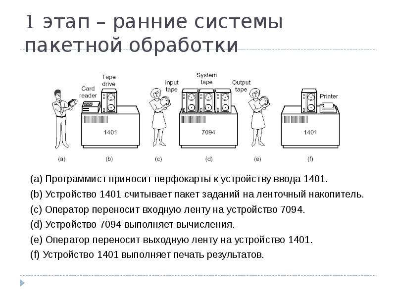
The solution to the problem was batch processing systems that provided centralized job collection on a separate device. This device read jobs from punch cards and recorded them on magnetic tape. When the magnetic tape with jobs was full, it was installed on a computer that sequentially read the jobs and executed them. The results of execution were recorded on a separate magnetic tape. The sequence of execution of tasks on the computer was controlled by a special program - monitor, the predecessor of modern operating systems. When the tape with the results of calculations was filled, it was removed from the computer and installed in a device that printed the results of calculations on punched cards or printed them on a printer.

The first GM-NAA batch processing system was implemented on an IBM 704 production system in 1955 by Robert Patrick of General Motors and Owen Mock of North American Aviation. In the image below you can see how the IBM 1401 batch data processing system was organized.

The use of batch processing reduced the downtime of computing machines waiting for jobs to load, which significantly improved their efficiency in scenarios where a large number of different tasks need to be performed.

1959: A Task Management Language

Batch processing tasks required certain data and output devices such as magnetic tapes, disk volumes, and printers. However, batch processing tools did not provide sufficient tools to provide all the resources needed by the task before the task started. As a result, "deadlock" situations could occur where job A holds resource R1 and requests resource R2, while simultaneously executing job B holds resource R2 and requests R1. In such cases, further execution of both jobs became impossible until the computer operator terminated the execution of one of the jobs to allow the other to continue, and then restarted the canceled job. It was necessary to improve the batch processing of jobs so that the resources and data sets it needed were clearly defined and a check was made on the availability of those resources and data before each task was started. This would prevent a task trying to use occupied resources from starting.

To solve the problem, the Job Control Language (JCL) was developed for late-model IBM mainframes of the IBM 7090 series and was widely used in the System/360 series. JCL unambiguously defined how to run a job or subsystem, which programs to run, which data sets or devices to use for input and output, and on which machine to run the job. The job scheduler that JCL worked with tracked and provided information about the resources used by the jobs. This allowed for optimized task execution, including the simultaneous execution of multiple jobs. For example, one program was waiting for input, another was actively working on the CPU, and a third was generating output. The scheduler also allowed to form queues for calculations with different data, add and delete tasks, change priorities and remove irrelevant tasks. JCL made it possible to organize work with mainframes through remote terminals, with the help of which it was possible to transfer a task and get the result of the program to output devices. These features already resembled modern client-server systems and allowed to use remote resources efficiently, improving the convenience of working with computing machines.

The relevance of job control languages was enhanced by the advent of hard disks in the mid-1950s, which provided fast random access to data. JCL allowed more efficient use of mainframe resources, which improved the performance and usability of computing machines. JCL was the progenitor of an ecosystem of job management tools, including schedulers and task optimization tools that have become the standard for many computing systems.

1969: ARPANET

The US Defense Advanced Research Projects Agency (ARPA, now called DARPA) created the Information Processing Techniques Office (IPTO) to conduct research into the conceptual aspects of military command and control. IPTO was headed by Carl Licklider, and who initiated the creation of computer science departments in several US universities.

Computer science departments and IPTO research laboratories of the time needed to be equipped with computing machines, but these were expensive and there were concerns that the demand for them might not be fully met. On the other hand, the existing computing machines were sometimes used inefficiently, left unused and idle. Licklider expressed the idea of combining heterogeneous computing resources into a single computing network with the division of access to machines by time. Also Licklider's idea was to remotely use the most efficient machines to solve a particular problem, given that the machines of the time were less versatile and often designed for narrow tasks. The prototype of such a network was the SAGE air defense data exchange network, which was used for military purposes and which Licklider was involved in creating.

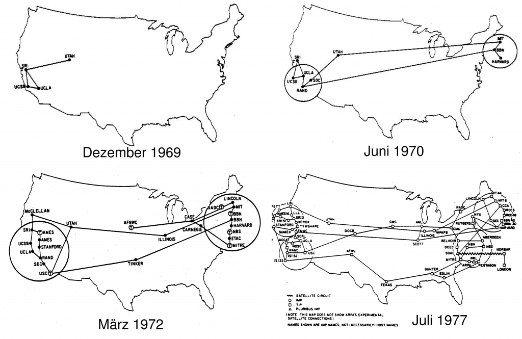
In 1964, practical work began on the realization of the network, which was called ARPANET. On October 29, 1969, for the first time it was possible to connect the computer of Stanford University, located at a distance of 600 km, with the computer of the California Institute of Technology. On the second attempt, the first message was transmitted: "login". Thus, the first ever users of the network were graduate students Charlie Kline, who transmitted the signal, and Bill Duvall, who received it.

In 1970, a network management protocol was implemented and the network was declared operational in 1971. Software development allowed remote login, file transfer and e-mail forwarding.

The creation of ARPANET provided the initial impetus for the development of the Internet, stimulated technological innovation, and provided a research environment for the development and improvement of computer networks, showing their feasibility and usefulness by inspiring researchers to interconnect computing machines into networks.

1969: Open Network Standards

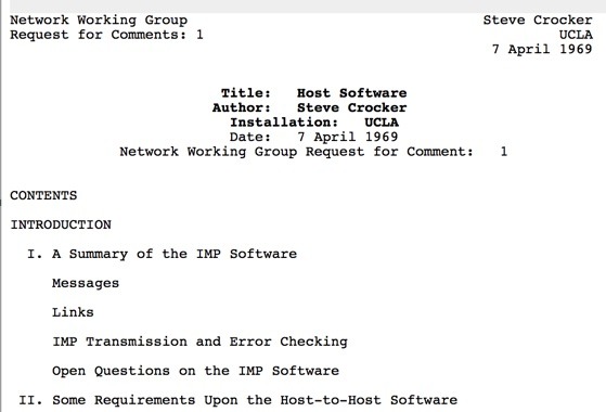
By the end of the 1960s, the U.S. was actively working to create the ARPANET network, which required standardization of formats, protocols, and procedures important for data exchange. And since at the dawn of computer network development there was no clear understanding of the best way to develop data exchange technologies, it was decided to first distribute the draft standards for discussion and feedback from the community, and then to approve them. This format of posting and discussing documents was called Request for Comments (RFC).

The first document, RFC 1, was published by Steve Crocker on April 7, 1969. This document presented an idea of how a new series of documents could be organized. Since then, RFCs have become the standard way of developing and documenting Internet protocols and specifications. RFCs are used to describe various aspects of networks and technologies and to discuss new ideas. RFCs are usually published and maintained by the Internet Engineering Task Force (IETF), and can be contributed to by any interested participant.

RFC allowed to bring order and standardize data exchange technologies and became a platform for discussion of new development concepts. RFC documents are now actively used and regulate Internet protocols, formats and standards. For example, RFC regulates the TCP/IP protocol (RFC1180) or the transmission of IP packets using carrier pigeons (RFC 1149).

1969: UNIX and C

In the 1960s, engineers' approaches to computer architecture were very different. Machines were built to solve certain tasks and optimized for these tasks. Each machine was developed with its own highly specialized operating systems that were incompatible with other machines and operating systems.

The PDP-7 18-bit computing machine was no exception, and when developing it, there was a need for a new operating system. Bell Labs was engaged to create an operating system for the PDP-7 machine. It was decided to build the operating system for the PDP-7 based on the Multics multitasking operating system developed by Bell Labs. The result of the development, completed in 1969, was a single-tasking OS, which was called Unics (later renamed Unix). Unics featured a modular architecture, consisting of a kernel that could be relatively easily adapted to run on different processors, and a set of utilities that could be modified or replaced separately from the kernel.

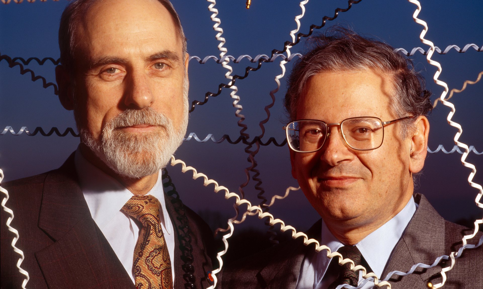
The creators of Unix, Ken Thompson and Dennis Ritchey, the men you see in the photo below, were concurrently developing a programming language that later became known as C. This language was a simplified version of the BCPL language. Currently, the proportion of server applications written in C and its variations is estimated at 30-50%. Various versions of Unix were rewritten in new versions of C, optimized and extended, becoming more flexible. And since Unix was originally designed to be a multitasking and multiuser operating system, it didn't take long for Unix to realize these properties. Since 1973, the source codes of the Unix operating system have been distributed to universities and academic institutions. The need to distribute Unix codes arose in order to make it a commercial product and to profit from solutions based on it. Such restrictions were necessary to circumvent the requirements of the agreement between the U.S. Department of Justice and AT&T, the owner of Bell Labs, which prohibited commercial activities unrelated to communication networks and equipment for them. The distribution of Unix source code set common standards and approaches for the industry, creating a Unix ecosystem and freeing the industry from a glut of incompatible solutions that hindered development as a whole.

Unix had a huge impact on the deployment of server applications by introducing new concepts and approaches such as hierarchical file system, OS modularity, command line, and text-based I/O orientation. Unix made the TCP/IP protocol possible on relatively inexpensive computers, leading to the rapid growth of computing networks. Many operating systems were developed based on Unix or were inspired by its architecture, such as Linux, macOS, iOS, Android, BSD, Solaris, AIX, and HP-UX. Currently, Unix-based systems and its variants such as Linux remain the primary operating systems for deploying server applications.

1973: International Data Network

As the first ARPANET connection outside the United States, a transatlantic cable connection was established with NORSAR of Norway in 1973. Around the same time, a link from Norway to London was installed. The lines had a data rate of 9.6 Kbps.

At first, the ARPANET connection to NORSAR was mainly used to exchange seismic data. As the network grew and new international links were established, NORSAR provided access to other Norwegian research organizations.

The establishment of an intercontinental connection between ARPANET and NORSAR was an important event that marked the beginning of the global network.

1974: TCP/IP

In the mid-1970s, in the early days of computer networking, there were several manufacturers of networking equipment that followed different standards and protocols for data transmission. There were also OSI specifications that you had to pay for the right to use when creating software.

There was a need for a common standard that would link devices from different manufacturers and would not be burdensome for enthusiasts. Transmission Control Protocol/Internet Protocol (TCP/IP) became such a standard, allowing networks of different types and manufacturers to successfully exchange information, providing the basis for the creation of the Internet.

In 1973, engineers Vince Cerf and Robert Kahn created the Transmission Control Protocol (TCP), which provided reliable data transmission in computer networks. TCP broke data into packets, monitored their transmission, and controlled the order in which they arrived at the destination. However, TCP was only part of the solution, and it lacked a description of how to route and identify nodes on the network.

To complement TCP, Vince Cerf and Robert Kahn developed the Internet Protocol (IP) in 1974. IP was responsible for addressing and routing data between network nodes. The combination of TCP and IP formed the basic TCP/IP protocol stack.

In 1981, the TCP and IP protocols were formalized and their specifications were published in RFC 793 for TCP and RFC 791 for IP. Gradually, networks using TCP/IP spread all over the world, and today TCP/IP are the main protocols of data exchange in the Internet, playing a crucial role in modern information infrastructure.

1983: Internet

In 1983, the ARPANET network switched from the NCP protocol to the TCP/IP protocol. By this time, the network had more than 4000 hosts, located mainly in the United States, and data transmission to Europe was carried out via cable lines and satellite links. With the transition to TCP/IP, ARPANET was moving from a centralized military network to a decentralized civilian structure in which different segments would be controlled by different organizations while maintaining connectivity. The defense-related segments of the network were separated into a separate network, MILNET. At this time, the ARPANET became known as the "Internet".

In 1984, the Domain Name System (DNS) was developed and a new inter-university network, NSFNet, was launched by the US National Science Foundation (NSF). NSFNet was created to link several U.S. supercomputer centers with universities, allowing scientists to work remotely with computing equipment. NSFNet was also intended to interconnect the CSNET and Bitnet scientific networks. NSFNet began operation in 1986 with six backbones with a bandwidth of 56 kbps. The agency then decided to expand the scope of NSFNet by allowing universities and schools to use it for other academic purposes, and to merge it with Usenet, which was used for news information. Schools that could not connect directly to NSFNet joined together to create regional networks, and together they connected to the NSFNet node, greatly expanding the reach of the network. NSFNet eventually absorbed all ARPANET hosts by 1990 and took the name "Internet" for itself.

NSFNet continues to exist and unites the computing power of supercomputers and universities around the world, including Moscow State University. On the basis of NSFNet, the Internet2 project is now being developed, which provides digital communication at high speeds. Internet2 - uses IPv6 protocol and multicast broadcasting, QoS support and the use of high-speed backbones of 100 Gbit/s and more.

1987: RAID

In the late 1980s, computing centers used SLED (Single Large Expensive Drive) form factor disks, which were significantly larger in size than personal computer disks. SLEDs had high performance, reliability, and high capacity, but their cost was very high. Despite the advantages, SLED disks were also prone to failures, albeit less frequently, and did not always have sufficient capacity and speed for some tasks.

To overcome the limitations of SLED, the concept of RAID (Redundant Array of Inexpensive Disks) was developed at UC Berkeley, involving an array of inexpensive personal computer disks served by a dedicated disk controller. RAID combines multiple physical disks into a single logical unit of storage using different levels or configurations, providing the benefits of increased reliability, improved performance, or a combination of both, depending on the RAID level selected.

The first RAID level, called "Mirroring", appeared in 1987. It involved creating mirror copies of data on two (or more) independent disks, providing data backup and protection against failure of one of the disks.

Subsequently, RAID levels such as RAID 2, RAID 3 and RAID 4 were introduced, which were not widely used. In 1990, RAID 5 and RAID 0 came out and became popular. RAID 5 provided efficient use of disks with data protection based on parity bits, while RAID 0 improved performance by splitting data between disks. As technology evolved, new RAID levels such as RAID 6, RAID 10, RAID 50 and others emerged, providing more complex and reliable storage configurations.

The use of RAID arrays has had a significant impact on improving storage performance, reducing the risks of data loss, and making information storage more accessible and reliable. Today, RAID controllers are widely used in servers, data warehouses and other systems where high reliability and performance are required.

1989: World Wide Web

At the end of the 1980s, the European Organization for Nuclear Research (CERN) had accumulated a huge amount of research information that needed to be accessed by staff within an intranet. Tim Berners-Lee proposed a solution to the problem of document organization: the creation of a distributed system of electronic documents - hypertexts linked to each other by hyperlinks, which would facilitate the search and consolidation of information. URI identifiers, the HTTP protocol and the HTML language were developed for the project, technologies that formed the basis of the modern Internet.

The project in 1989 was called World Wide Web (WWW) and implied a global focus beyond the internal CERN network. The need for a global system was present because the research documents of the international CERN were demanded by scientists from many countries.

Improvement of standards and protocols continued until 1993, when they were published. And in 1994, the World Wide Web Consortium (W3C) was created by Tim Berners-Lee to take responsibility for developing, implementing, and promoting open standards that provide access to the World Wide Web.

1991: First Internet Server

On August 6, 1991, the first web site was created, hosted by the creator of the WWW project, Berners-Lee. To make the site work, the HTTPD web server was developed, and the WorldWideWeb browser, which was also the editor of HTML documents.

The site can still be found at https://info.cern.ch/. This resource defines the WWW, provides instructions on installing a web server and using a browser.

Within two years after the first web site appeared, the number of web sites on the WWW reached 200 and continued to grow. Today, there are about two billion websites on the WWW.

1993: Imperative Configuration Managers

Version control systems date back to the mainframe era in the late 1950s and early 1960s, such as CDC UPDATE and IBM IEB_UPDATE. These systems allowed software components to be automatically updated and modified. But over time, information systems became increasingly complex, including not only code but also various configuration files, resources, customizations, etc. The increased complexity of systems when configured manually increased the risks of configuration errors, as well as the appearance of heterogeneity and inconsistencies in configurations. While the growth of the computing fleet in the 1990s required more and more effort from the staff to maintain the right computing configuration. Automated mass monitoring and configuration tools were required to address this problem.

The first configuration management system, CFEngine, was developed by Mark Burgess and appeared in 1993. Mark Burgess was faced with the task of automating the management of a small group of workstations running on different platforms. Writing scripts to troubleshoot user problems was becoming too time-consuming, and the differences in platforms and Unix versions required a customized approach. To solve this problem, CFEngine was developed to help smooth out platform differences through its object-oriented language. The tool was small, resource-efficient, and could continue configuration even if communication with the controlling machine was lost.

In 1994, a Perl-based configuration management system, LCFG, was created at the University of Edinburgh to manage a fleet of computing equipment. LCFG allowed nodes to request configuration from the host computer and update it according to a specified profile. This system was applied to networks with diverse and rapidly changing configurations.

From 1998, various configuration management managers such as ISConf, PIKT and STAF started to appear. ISConf was suitable for homogeneous environments where identical configurations had to be maintained. PIKT focused on state monitoring and could also manage configurations. STAF, developed by IBM in C++, specialized in automating the configuration of test environments for software development and supported different platforms and operating system versions.

Bcfg2 configuration manager was developed at Argonne National Laboratory in 2002. Bcfg2 focused on auditing the current configuration and alerting on violations of specified parameters. It was written in Python and gained popularity among Python programmers.

Also in 2002, ISConf 3 was released, written in Perl by Luke Cañez based on ISConf 2. After the completion of ISConf 3, Luc Cañez got involved in the development of CFEngine 2, which came out in 2002 under the direction of Mark Burgess. CFEngine 2 introduced the concept of declarative description of the desired system state and system self-healing. The experience of the development of ISConf 3 and CFEngine 2 by Luke Cañez will form the basis for the development of Puppet.

In 2003, based on the LCFG manager architecture, the Quattor manager was created as part of the European Data Grid distributed computing project. Quattor was used to install, configure and manage computers and allowed to use a variety of configuration templates based on hierarchical blocks written in Pan language.

The same year saw the introduction of Radmind, a manager developed for Mac OS X systems. Its purpose was to track changes in the file system and the ability to undo those changes.

In January 2004, HP made the source code for its SmartFrog distributed platform, written in Java, publicly available. SmartFrog was intended to simplify and automate the design, configuration, deployment, and management of distributed systems. SmartFrog had its own: language, runtime environment, and component library.

Also in 2004, Synctool, a configuration management manager written in Python, appeared. It was focused on ease of use and used SSH and rsync to connect. Synctool did not require a special language for configuration and scripts could be written in any scripting language.

In 2005, the Capistrano tool written in Ruby by Jamis Buck and Lee Hamblin was introduced. Capistrano is designed to deploy and manage web applications on remote servers created using the Ruby on Rails framework or the PHP language. Capistrano continues to be maintained and updated, with the last version I noticed released in May 2023.

The first configuration managers were designed to track changes to the initial configuration and return it to its initial state. Alternatively, they were imperative, requiring scripts to be provided to define a sequence of actions from the initial state to the desired end state. However, this approach had the disadvantage of requiring an accurate understanding of the initial state of the system in order to properly build a sequence of actions leading to the desired end state and a customized approach for each initial state. However, CFEngine 2 began to introduce mechanisms for declarative description of the desired system state, which led to a qualitative improvement of configuration management managers and made them what we see today. Despite the limitations of functionality in the initial stages of development, configuration managers have greatly facilitated administration and have become the basis for the development of modern declarative configuration managers and deployment tools.

Of course, the development of configuration management tools has continued, including the development of the imperative approach. However, in an article about traditional deployment, I would like to limit my discussion to the period before Puppet was released, which came out in 2005, set some standards, and made much of what had been created before obsolete. I will talk about Puppet, what comes after Puppet, and the declarative approach in general in the next article on the history of virtual deployment, as I feel that these topics will be more relevant there.

1995: Java and PHP

In the mid-90s, the popularity of the Internet was growing rapidly and more developers started to develop applications for the Internet, but there was a lack of simple and effective tools for developing web applications, especially cross-platform ones. The tools and solutions that existed at that time were difficult to learn, not very efficient or had difficulties with scaling and working on different platforms.

Enthusiasts have also tried to solve the problem of insufficient web development tools. One such enthusiast, Danish programmer Rasmus Lerdorf, developed a set of C scripts to track visits to his online resume and personal web page statistics. He called his simple and effective set "Personal Home Page Tools". In 1995, Rasmus published the source code for an extended version of his toolkit, which he called "PHP/FI" (Personal Home Page/Forms Interpreter). PHP/FI added support for working with databases and HTML forms.

The development community saw the potential in PHP and began to actively add new functionality to it. Its ease of learning, broad support from hosting providers, large developer community, and ease of data processing and database integration have made PHP one of the most popular programming languages for creating dynamic web applications.

Comparatively simple syntax and versatility allowed another programming language to become popular, which started to be developed in the early 1990s by a team from Sun Microsystems, led by James Gosling. The new programming language Oak was to be simple, reliable, scalable and cross-platform. The development of Oak was completed in 1995 and it was introduced to the public under the name Java, and with it the Java Application Development Kit (JDK). The Java language is focused on the development of "applets" (applets), which are small interactive applications that run in web browsers. Comparatively simple Java syntax, extensive library of standard functions and tools allowed to easily create cross-platform applications, and security mechanisms, high reliability and scalability allowed to realize large enterprise-level projects. The Java language has become one of the main programming languages in the industry and is used to develop a variety of applications from mobile to server applications.

The simple syntax and versatility of Java and PHP made web development easier, which attracted many developers, especially beginners, and positively influenced the development of server-side deployment.  Java and PHP have become more attractive compared to other less beginner-friendly languages such as Perl and C. The popularity of Java and PHP increased rapidly during the dot-com bubble, when the demand for web application developers was very high, and rapid adoption of web development languages became a very important factor.

2000: Web-API

Mechanisms, interaction of program components - APIs appeared at the dawn of computing technology, in the 40s, although the very definition of API (application programming interface) appeared decades later.

The API provided a standardized interface for interaction and data exchange between programs and services on a single computing machine without the need to understand the internal structure and mechanisms of the component with which the interaction takes place. This helped developers to use the functionality of other components with minimal effort to learn how they work.

With the advent of Internet servers, there was a need to organize interaction with their functionality, and the application of API principles became an obvious solution. This solution was called Web-API.

The first Web-API was introduced by Salesforce.com on February 7, 2000, but these APIs were not publicly available and were not intended to be publicly accessible. The main role of these APIs was to allow customer business applications to exchange data with each other.

About 9 months later, eBay launched its API - eBay Application Program Interface along with the eBay Developers Program, making the first API open to developers.

Web-API provided an effective tool that provided a standardized way for clients and servers to interact over the network. This made it easy for developers to create flexible, scalable, and cross-platform web services for data exchange and remote operations.

What's the Bottom Line?

The emergence of servers has played a huge role in the development of information technology, providing an opportunity to centralize the placement of information and its processing. Centralized data processing and storage made it possible to simplify data management, increase computing efficiency, and ensure high reliability and security of data storage. Instead of storing all data and applications on users' computers, some of it began to be stored and processed on servers, making data handling more convenient and efficient. Most of us no longer store music, photos, and program distributions in our archives on removable media as we used to, all of this data has moved to servers. Some software has also moved to servers; for example, we can type or create a spreadsheet through Google docs, we can recognize text or translate it into another language online.

With the advent of servers, it became possible to create complex distributed computing systems, data storage systems and services that can be accessed remotely from anywhere in the world. Servers became the foundation for the development of various technologies and solutions in the IT industry - from corporate information systems and databases to web servers, data warehouses and web services.

Traditional deployment of server-based applications was the first and, unfortunately, was not free of drawbacks. However, its emergence served as a starting point for the development of other types of deployments, the history of which we will describe in the following articles. In the meantime, to understand the differences going forward, let's define what traditional application deployment is and what its weaknesses and strengths are.

In traditional deployment, server applications are deployed directly to the physical server whose operating system is managed. Along with the application, its dependencies, such as external libraries, frameworks, modules, and data required for operation, are installed on the server. Traditional deployment uses relatively simple software for installation and load management; virtualization and containerization systems are not used, which somewhat reduces staff skill requirements. The absence of an additional layer of abstraction in the form of virtualization or containerization systems ensures direct interaction with hardware and minimal latency.

Traditional deployment can also be applied in the case of client-server architecture, where the frontend is deployed on client devices and the backend and database on servers. In this model, client devices access the server to retrieve data and execute business logic.

The main disadvantage of traditional deployment is its low flexibility. When the application load increases, additional hardware is required, resulting in time and resources spent configuring and installing it. When the load decreases, resources can become idle, reducing the efficiency of hardware utilization. Managing server resources and configuration in a traditional deployment requires individually configuring and maintaining each server separately, which can be a time-consuming task without the use of automation tools. In addition, management in a traditional software deployment approach often requires manual intervention, and if a rollback to a previous version of software is required, a backup or recreation of a previous working version of the entire system will be required. Overall, traditional deployment does not appear to be convenient or efficient from an administrative perspective.

In general, the traditional deployment method may be suitable for small projects with limited resource requirements with predictable load levels, as well as for specialized tasks, including some High-load systems, where it is necessary to ensure minimum latency in information processing. But traditional deployment will inevitably become a limiting factor when developing and scaling complex and distributed systems.

To summarize, the traditional approach is characterized by the need for dedicated hardware, low flexibility, limited scalability and high operating costs. As the demand for compute and storage grows, this approach is only justified for a narrow range of applications.

In the following installments, I will discuss how the IT industry has tried to overcome the shortcomings of traditional deployment with virtual and containerized deployment.